As businesses grow with larger customers size and hire more employees, they face challenges to meet the customer demands in terms of scaling their systems and maintaining rapid product development with bigger teams. The businesses aim to scale systems linearly with additional computing and human resources. However, systems architecture such as monolithic or ball of mud makes scaling systems linearly onerous. Similarly, teams become less efficient as they grow their size and become silos. A general solution to solve scaling business or technical problems is to use divide & conquer and partition it into multiple sub-problems. A number of factors affect scalability of software architecture and organizations such as the interactions among system components or communication between teams. For example, the coordination, communication and data/knowledge coherence among the system components and teams become disproportionately expensive with the growth in size. The software systems and business management have developed a number of laws and principles that can used to evaluate constraints and trade offs related to the scalability challenges. Following is a list of a few laws from the technology and business domain for scaling software architectures and business organizations:
Amdhal’s Law
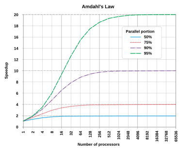
Amdahl’s Law is named after Gene Amdahl that is used to predict speed up of a task execution time when it’s scaled to run on multiple processors. It simply states that the maximum speed up will be limited by the serial fraction of the task execution as it will create resource contention:
Speed up (P, N) = 1 / [ (1 - P) + P / N ]
Where P is the fraction of task that can run in parallel on N processors. When N becomes large, P / N approaches 0 so speed up is restricted to 1 / (1 – P) where the serial fraction (1 – P) becomes a source of contention due to data coherence, state synchronization, memory access, I/O or other shared resources.
Amdahl’s law can also be described in terms of throughput using:
N / [ 1 + a (N - 1) ]
Where a is the serial fraction between 0 and 1. In parallel computing, a class of problems known as embarrassingly parallel workload where the parallel tasks have a little or no dependency among tasks so their value for a will be 0 because they don’t require any inter-task communication overhead.
Amdah’s law can be used to scale teams as an organization grows where the teams can be organized as small and cross-functional groups to parallelize the feature work for different product lines or business domains, however the maximum speed up will still be limited by the serial fraction of the work. The serial work can be: build and deployment pipelines; reviewing and merging changes; communication and coordination between teams; and dependencies for deliverables from other teams. Fred Brooks described in his book The Mythical Man-Month how adding people to a highly divisible task can reduce overall task duration but other tasks are not so easily divisible: while it takes one woman nine months to make one baby, “nine women can’t make a baby in one month”.
Brooks’s Law
Brooks’s law was coined by Fred Brooks that states that adding manpower to a late software project makes it later due to ramp up time. As the size of team increases, the ramp up time for new employees also increases due to quadratic communication overhead among team members, e.g.
Number of communication channels = N x (N - 1) / 2
The organizations can build small teams such as two-pizza/single-threaded teams where communication channels within each team does not explode and the cross-functional nature of the teams require less communication and dependencies from other teams. The Brook’s law can be equally applied to technology when designing distributed services or components so that each service is designed as a loosely coupled module around a business domain to minimize communication with other services and services only communicate using a well designed interfaces.
Universal Scalability Law
The Universal Scalability Law is used for capacity planning and was derived from Amdahl’s law by Dr. Neil Gunther. It describes relative capacity in terms of concurrency, contention and coherency:
C(N) = N / [1 + a(N – 1) + B.N (N – 1) ]
Where C(N) is the relative capacity, a is the serial fraction between 0 and 1 due to resource contention and B is delay for data coherency or consistency. As data coherency (B) is quadratic in N so it becomes more expensive as size of N increases, e.g. using a consensus algorithm such as Paxos is impractical to reach state consistency among large set of servers because it requires additional communication between all servers. Instead, large scale distributed storage services generally use sharding/partitioning and gossip protocol with a leader-based consensus algorithm to minimize peer to peer communication.
The Universal Scalability Law can be applied to scale teams similar to Amdahl’s law where a is modeled for serial work or dependency between teams and B is modeled for communication and consistent understanding among the team members. The cost of B can be minimized by building cross-functional small teams so that teams can make progress independently. You can also apply this model for any decision making progress by keeping the size of stake holders or decision makers small so that they can easily reach the agreement without grinding to halt.
The gossip protocols also applies to people and it can be used along with a writing culture, lunch & learn and osmotic communication to spread knowledge and learnings from one team to other teams.
Little’s Law
Little’s Law was developed by John Little to predict number of items in a queue for stable stable and non-preemptive. It is part of queueing theory and is described mathematically as:
L = A W
Where L is the average number of items within the system or queue, A is the average arrival time of items and W is the average time an item spends in the system. The Little’s law and queuing theory can be used for capacity planning for computing servers and minimizing waiting time in the queue (L).
The Little’s law can be applied for predicting task completion rate in an agile process where L represents work-in-progress (WIP) for a sprint; A represents arrival and departure rate or throughput/capacity of tasks; W represents lead-time or an average amount of time in the system.
WIP = Throughput x Lead-Time
Lead-Time=WIP / Throughput
You can use this relationship to reduce the work in progress or lead time and improve throughput of tasks completion. Little’s law observes that you can accomplish more by keeping work-in-progress or inventory small. You will be able to better respond to unpredictable delays if you keep a buffer in your capacity and avoid 100% utilization.
King’s formula
The King’s formula expands Little’s law by adding utilization and variability for predicting wait time before serving of requests:

where T is the mean service time, m (1/T) is the service rate, A is the mean arrival rate, p = A/m is the utilization, ca is the coefficient of variation for arrivals and cs is the coefficient of variation for service times. The King’s formula shows that the queue sizes increases to infinity as you reach 100% utilization and you will have longer queues with greater variability of work. These insights can be applied to both technical and business processes so that you can build systems with a greater predictability of processing time, smaller wait time E(W) and higher throughput ?.
Note: See Erlang analysis for serving requests in a system without a queue where new requests are blocked or rejected if there is not sufficient capacity in the system.
Gustafson’s Law
Gustafson’s law improves Amdahl’s law with a keen observation that parallel computing enables solving larger problems by computations on very large data sets in a fixed amount of time. It is defined as:
S = s + p x N
S = (1 – s) x N
S = N + (1 – N) x s
where S is the theoretical speed up with parallelism, N is the number of processors, s is the serial fraction and p is the parallel part such that s + p = 1.
Gustafson’s law shows that limitations imposed by the sequential fraction of a program may be countered by increasing the total amount of computation. This allows solving bigger technical and business problems with a greater computing and human resources.
Conway’s Law
Conway’s law states that an organization that designs a system will produce a design whose structure is a copy of the organization’s communication structure. It means that the architecture of a system is derived from the team structures of an organization, however you can also use the architecture to derive the team structures. This allows defining building teams along the architecture boundaries so that each team is a small, cross functional and cohesive. A study by the Harvard Business School found that the often large co-located teams tended to produce more tightly-coupled and monolithic codebases whereas small distributed teams produce more modular codebases. These lessons can be applied to scaling teams and architecture so that teams and system modules are built around organizational boundaries and independent concerns to promote autonomy and reduce tight coupling.
Pareto Principle
The Pareto principle states that for many outcomes, roughly 80% of consequences come from 20% of causes. This principle shows up in numerous technical and business problems such as 20% of code has the 80% of errors; customers use 20% of functionality 80% of the time; 80% of optimization improvements comes from 20% of the effort, etc. It can also be used to identify hotspots or critical paths when scaling, as some microservices or teams may receive disproportionate demands. Though, scaling computing resources is relatively easy but scaling a team beyond an organization boundary is hard. You will have to apply other management tools such as prioritization, planning, metrics, automation and better communication to manage critical work.
Metcalfe’s Law
The Metcalfe’s law states that if there are N users of a telecommunications network, the value of the network is N2. It’s also referred as Network effects and applies to social networking sites.
Number of possible pair connections = N * (N – 1) / 2
Reed’s Law expanded this law and observed that the utility of large networks can scale exponentially with the size of the network.
Number of possible subgroups of a network = 2N – N – 1
This law explains the popularity of social networking services via viral communication. These laws can be applied to model information flow between teams or message exchange between services to avoid peer to peer communication with extremely large group of people or a set of nodes. A common alternative is to use a gossip protocol or designate a partition leader for each group that communicates with other leaders and then disseminate information to the group internally.
Dunbar Number
The Dunbar’s number is a suggested cognitive limit to the number of people with whom one can maintain stable social relationships. It has a commonly used value of 150 and can be used to limit direct communication connections within an organization.
Wirth’s Law and Parkinson’s Law
The Wirth’s Law is named after Niklaus Wirth who observed that the software is getting slower more rapidly than hardware is becoming faster. Over the last few decades, processors have become exponentially faster as a Moor’s Law but often that gain allows software developers to develop more complex software that consumes all gains of the speed. Another factor is that it allows software developers to use languages and tools that may not generate more efficient code so the code becomes bloated. There is a similar law in software development called Parkinson’s law that work expands to fill the time available for it. Though, you also have to watch for Hofstadter’s Law that states that “it always takes longer than you expect, even when you take into account Hofstadter’s Law”; and Brook’s Law, which states that “adding manpower to a late software project makes it later.”
The Wirth’s Law, named after Niklaus Wirth, posits that software tends to become slower at a rate that outpaces the speed at which hardware becomes faster. This observation reflects a trend where, despite significant advancements in processor speeds as predicted by Moor’s Law , software complexity increases correspondingly. Developers often leverage these hardware improvements to create more intricate and feature-rich software, which can negate the hardware gains. Additionally, the use of programming languages and tools that do not prioritize efficiency can lead to bloated code.
In the realm of software development, there are similar principles, such as Parkinson’s law, which suggests that work expands to fill the time allotted for its completion. This implies that given more time, software projects may become more complex or extended than initially necessary. Moreover, Hofstadter’s Law offers a cautionary perspective, stating, “It always takes longer than you expect, even when you take into account Hofstadter’s Law.” This highlights the often-unexpected delays in software development timelines. Brook’s Law further adds to these insights with the adage, “Adding manpower to a late software project makes it later.” These laws collectively emphasize that the demand upon a resource tends to expand to match the supply of the resource but adding resources later also poses challenges due to complexity in software development and project management.
Principle of Priority Inversion
In modern operating systems, the concept of priority inversion arises when a high-priority process needs resources or data from a low-priority process, but the low-priority process never gets a chance to execute due to its lower priority. This creates a deadlock or inefficiency where the high-priority process is blocked indefinitely. To avoid this, schedulers in modern operating systems adjust the priority of the lower-priority process to ensure it can complete its task and release the necessary resources, allowing the high-priority process to continue.
This same principle applies to organizational dynamics when scaling teams and projects. Imagine a high-priority initiative that requires collaboration from another team whose priorities do not align. Without proper coordination, the team working on the high-priority initiative may never get the support they need, leading to delays or blockages. Just as in operating systems, where a priority adjustment is needed to keep processes running smoothly, organizations must also ensure alignment across teams by managing a global list of priorities. A solution is to maintain a global prioritized list of projects that is visible to all teams. This ensures that the most critical initiatives are recognized and appropriately supported by every team, regardless of their individual workloads. This centralized prioritization ensures that teams working on essential projects can quickly receive the help or resources they need, avoiding bottlenecks or deadlock-like situations where progress stalls because of misaligned priorities.
Load Balancing (Round Robin, Least Connection)
Load balancing algorithms distribute tasks across multiple servers to optimize resource utilization and prevent any single server from becoming overwhelmed. Common strategies include round-robin (distributing tasks evenly across servers) and least connection (directing new tasks to the server with the fewest active connections).
Load balancing can be applied to distribute work among teams or individuals. For instance, round-robin can ensure that tasks are equally assigned to team members, while the least-connection principle can help assign tasks to those with the lightest workload, ensuring no one is overloaded. This leads to more efficient task management, better resource allocation, and balanced work distribution.
MapReduce
MapReduce splits a large task into smaller sub-tasks (map step) that can be processed in parallel, then aggregates the results (reduce step) to provide the final output. In a large project, teams or individuals can be assigned sub-tasks that they can work on independently. Once all the sub-tasks are complete, the results can be aggregated to deliver the final outcome. This fosters parallelism, reduces bottlenecks, and allows for scalable team collaboration, especially for large or complex projects.
Deadlock Prevention (Banker’s Algorithm)
The Banker’s Algorithm is used to prevent deadlocks by allocating resources in such a way that there is always a safe sequence of executing processes, avoiding circular wait conditions. In managing interdependent teams or tasks, it’s important to avoid deadlocks where teams wait on each other indefinitely. By proactively ensuring that resources (e.g., knowledge, tools, approvals) are available before committing teams to work, project managers can prevent deadlock scenarios. Prioritizing resource allocation and anticipating dependencies can ensure steady progress without one team stalling another.
Consensus Algorithms (Paxos, Raft)
Consensus algorithms ensure that distributed systems agree on a single data value or decision, despite potential failures. Paxos and Raft are used to maintain consistency across distributed nodes. In projects involving multiple stakeholders or teams, reaching consensus on decisions can be challenging, especially with different priorities and viewpoints. Consensus-building techniques, inspired by these algorithms, could involve ensuring that key stakeholders agree before any significant action is taken, much like how Paxos ensures agreement across distributed systems. This avoids misalignment and fosters collaboration and trust across teams.
Rate Limiting
Rate limiting controls the number of requests or operations that can be performed in a given timeframe to prevent overloading a system. This concept applies to managing expectations, particularly in teams with multiple incoming requests. Rate limiting can be applied to protect teams from being overwhelmed by too many requests at once. By limiting how many tasks or requests a team can handle at a time, project managers can ensure a sustainable work pace and prevent burnout, much like how rate limiting helps protect system stability.
Summary
Above laws offer strategies for optimizing both technical systems and team dynamics. Amdahl’s Law and the Universal Scalability Law highlight the challenges of parallelizing work, emphasizing the need to manage coordination and communication overhead as bottlenecks when scaling teams or systems. Brook’s and Metcalfe’s Laws reveal the exponential growth of communication paths, suggesting that effective team scaling requires managing these paths to avoid coordination paralysis. Little’s Law and Kingman’s Formula suggest limiting work in progress and preventing 100% resource utilization to ensure reliable throughput, while Conway’s Law underscores the alignment between team structures and system architecture. Teams and their responsibilities should mirror modular architectures, fostering autonomy and reducing cross-team dependencies.
The Pareto Principle can guide teams to make small but impactful changes in architecture or processes that yield significant productivity improvements. Wirth’s Law and Parkinson’s Law serve as reminders to prevent work bloat and unnecessary complexity by setting clear deadlines and objectives. Dunbar’s Number highlights the human cognitive limit in maintaining external relationships, suggesting that team dependencies should be kept minimal to maintain effective collaboration. The consensus algorithms used in distributed systems can be applied to decision-making and collaboration, ensuring alignment among teams. Error correction algorithms are useful for feedback loops, helping teams iteratively improve. Similarly, techniques like load balancing strategies can optimize task distribution and workload management across teams.
Before applying these laws, it is essential to have clear goals, metrics, and KPIs to measure baselines and improvements. Prematurely implementing these scalability strategies can exacerbate issues rather than resolve them. The focus should be on global optimization of the entire organization or system, rather than focusing on local optimizations that don’t align with broader goals.