Introduction
Building distributed systems means confronting failure modes that are nearly impossible to reproduce in development or testing environments. How do you test for metastable failures that only emerge under specific load patterns? How do you validate that your quorum-based system actually maintains consistency during network partitions? How do you catch cross-system interaction bugs when both systems work perfectly in isolation? Integration testing, performance testing, and chaos engineering all help, but they have limitations. For the past few years, I’ve been using simulation to validate boundary conditions that are hard to test in real environments. Interactive simulators let you tweak parameters, trigger failure scenarios, and see the consequences immediately through metrics and visualizations.
In this post, I will share four simulators I’ve built to explore the failure modes and consistency challenges that are hardest to test in real systems:
- Metastable Failure Simulator: Demonstrates how retry storms create self-sustaining collapse
- CAP/PACELC Consistency Simulator: Shows the real tradeoffs between consistency, availability, and latency
- CRDT Simulator: Explores conflict-free convergence without coordination
- Cross-System Interaction (CSI) Failure Simulator: Reveals how correct systems fail through their interactions
Each simulator is built on research findings and real-world incidents. The goal isn’t just to understand these failure modes intellectually, but to develop intuition through experimentation. All simulators available at: https://github.com/bhatti/simulators.
Part 1: Metastable Failures
The Problem: When Systems Attack Themselves
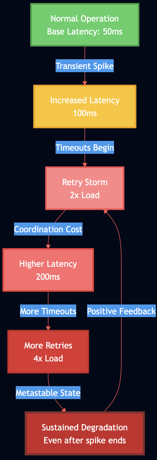
Metastable failures are particularly insidious because the initial trigger can be small and transient, but the system remains degraded long after the trigger is gone. Research in the metastable failures has shown that traditional fault tolerance mechanisms don’t protect against metastability because the failure is self-sustaining through positive feedback loops in retry logic and coordination overhead. The mechanics are deceptively simple:
- A transient issue (network blip, brief CPU spike) causes some requests to slow down
- Slow requests start timing out
- Clients retry timed-out requests, adding more load
- Additional load increases coordination overhead (locks, queues, resource contention)
- Higher overhead increases latency further
- More timeouts trigger more retries
- The system is now in a stable degraded state, even though the original trigger is gone
For example, AWS Kinesis experienced a 7+ hour outage in 2020 where a transient metadata mismatch triggered retry storms across the fleet. Even after the original issue was fixed, the retry behavior kept the system degraded. The recovery required externally rate-limiting client retries.
How the Simulator Works
The metastable failure simulator models this feedback loop using discrete event simulation (SimPy). Here’s what it simulates:
Server Model:
- Base latency: Time to process a request with no contention
- Concurrency slope: Additional latency per concurrent request (coordination cost)
- Capacity: Maximum concurrent requests before queueing
# Latency grows linearly with active requests
def current_latency(self):
    return self.base_latency + (self.active_requests * self.concurrency_slope)
Client Model:
- Timeout threshold: When to give up on a request
- Max retries: How many times to retry
- Backoff strategy: Exponential backoff with jitter (configurable)
Load Patterns:
- Constant: Steady baseline load
- Spike: Sudden increase for a duration, then back to baseline
- Ramp: Gradual increase and decrease
Key Parameters to Experiment With:
| Parameter | What It Tests | Typical Values |
|---|---|---|
server_capacity | How many concurrent requests before queueing | 20-100 |
base_latency | Processing time without contention | 0.1-1.0s |
concurrency_slope | Coordination overhead per request | 0.001-0.05s |
timeout | When clients give up | 1-10s |
max_retries | Retry attempts before failure | 0-5 |
backoff_enabled | Whether to add jitter and delays | True/False |
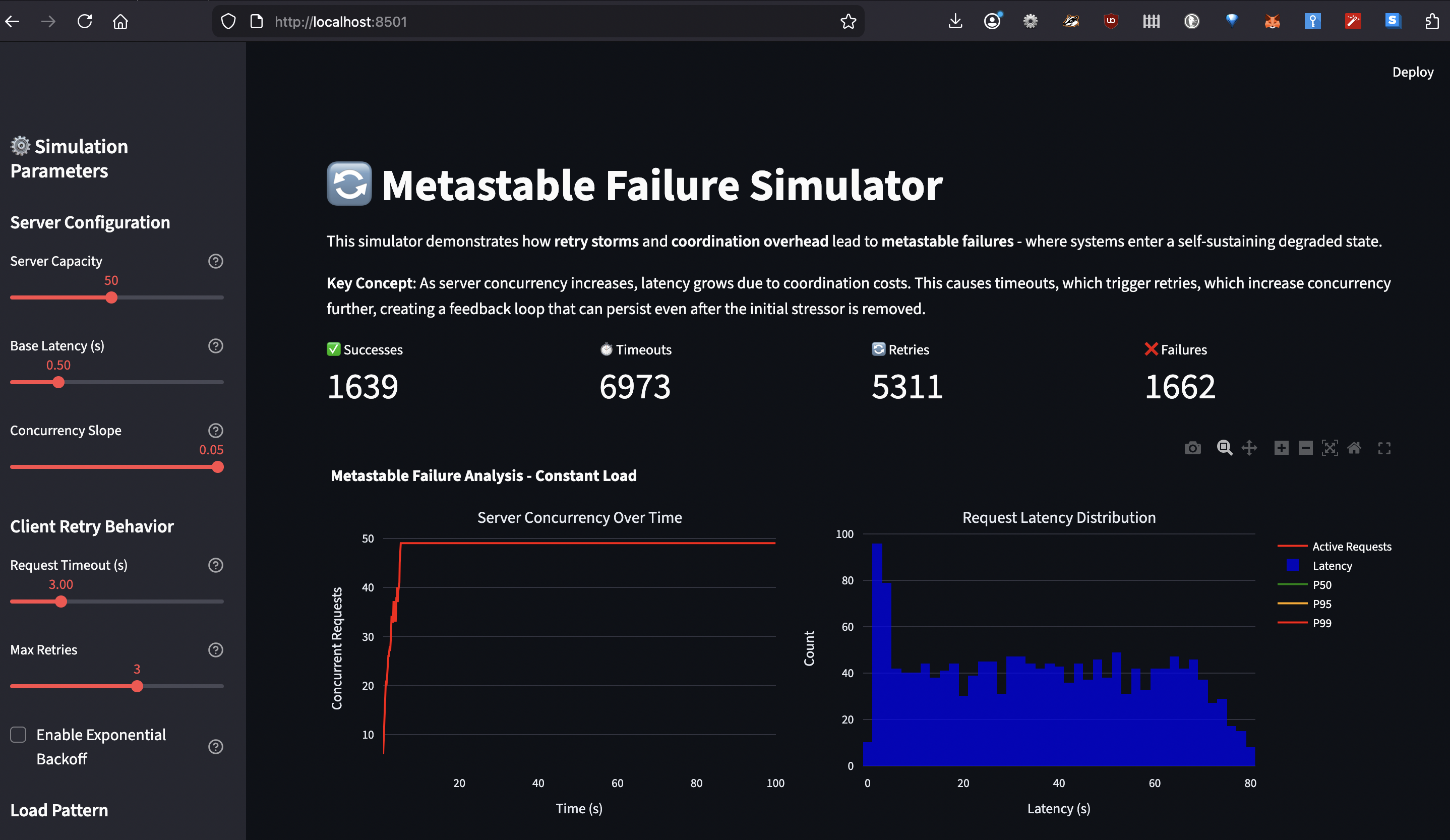
What You Can Learn:
- Trigger a metastable failure: Set spike load high, timeout low, disable backoff ? watch P99 latency stay high after spike ends
- See recovery with backoff: Same scenario but enable exponential backoff ? system recovers when spike ends
- Understand the tipping point: Gradually increase concurrency slope ? observe when retry amplification begins
- Test admission control: Set low server capacity ? see benefit of failing fast vs queueing
The simulator tracks success rate, retry count, timeout count, and latency percentiles over time, letting you see exactly when the system tips into metastability and whether it recovers. With this simulator you can validate various prevention strategies such as:
- Exponential backoff with jitter spreads retries over time
- Adaptive retry budgets limit total fleet-wide retries
- Circuit breakers detect patterns and stop retry storms
- Load shedding rejects requests before queues explode
Part 2: CAP and PACELC
The CAP theorem correctly states that during network partitions, you must choose between consistency and availability. However, as Daniel Abadi and others have pointed out, this only addresses partition scenarios. Most systems spend 99.99% of their time in normal operation, where the real tradeoff is between latency and consistency. This is where PACELC comes in:
- If Partition happens: choose Availability or Consistency
- Else (normal operation): choose Latency or Consistency
PACELC provides a more complete framework for understanding real-world distributed databases:
PA/EL Systems (DynamoDB, Cassandra, Riak):
- Partition ? Choose Availability (serve stale data)
- Normal ? Choose Latency (1-2ms reads from any replica)
- Use when: Shopping carts, session stores, high write throughput needed
PC/EC Systems (Google Spanner, VoltDB, HBase):
- Partition ? Choose Consistency (reject operations)
- Normal ? Choose Consistency (5-100ms for quorum coordination)
- Use when: Financial transactions, inventory, anything that can’t be wrong
PA/EC Systems (MongoDB):
- Partition ? Choose Availability (with caveats – unreplicated writes go to rollback)
- Normal ? Choose Consistency (strong reads/writes in baseline)
- Use when: Mixed workloads with mostly consistent needs
PC/EL Systems (PNUTS):
- Partition ? Choose Consistency
- Normal ? Choose Latency (async replication)
- Use when: Read-heavy with timeline consistency acceptable
Quorum Consensus: Strong Consistency with Coordination
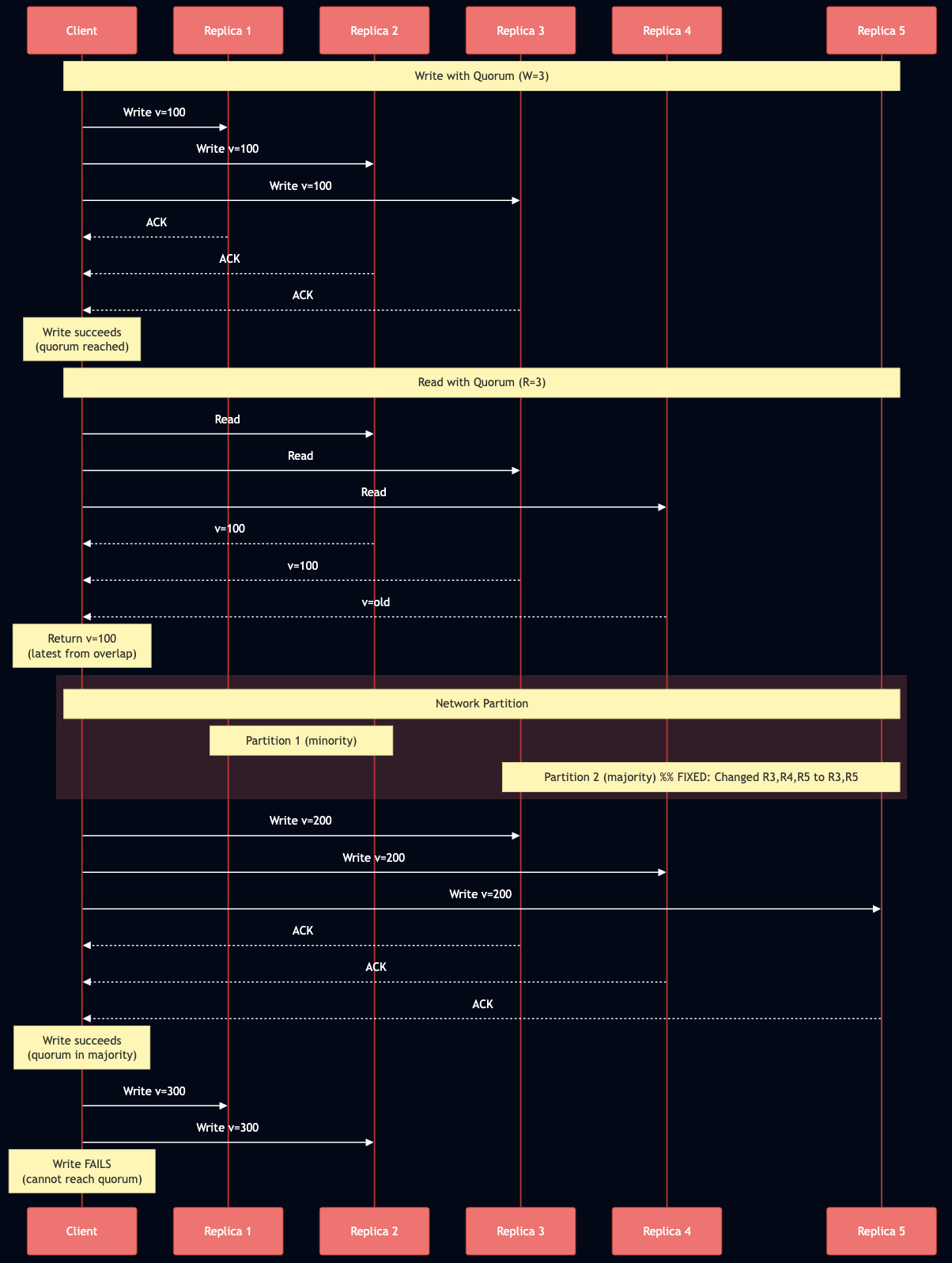
When R + W > N (read quorum + write quorum > total replicas), the read and write sets must overlap in at least one node. This overlap ensures that any read sees at least one node with the latest write, providing linearizability.
Example with N=5, R=3, W=3:
- Write to replicas {1, 2, 3}
- Read from replicas {2, 3, 4}
- Overlap at {2, 3} guarantees we see the latest value
Critical Nuances:
R + W > N alone is NOT sufficient for linearizability in practice. You need additional mechanisms: readers must perform read repair synchronously before returning results, and writers must read the latest state from a quorum before writing. “Last write wins” based on wall-clock time breaks linearizability due to clock skew. Sloppy quorums like those used in Dynamo are NOT linearizable because the nodes in the quorum can change during failures. Even R = W = N doesn’t guarantee consistency if cluster membership changes. Google Spanner uses atomic clocks and GPS to achieve strong consistency globally, with TrueTime API providing less than 1ms clock uncertainty at the 99th percentile as of 2023.
How the Simulator Works
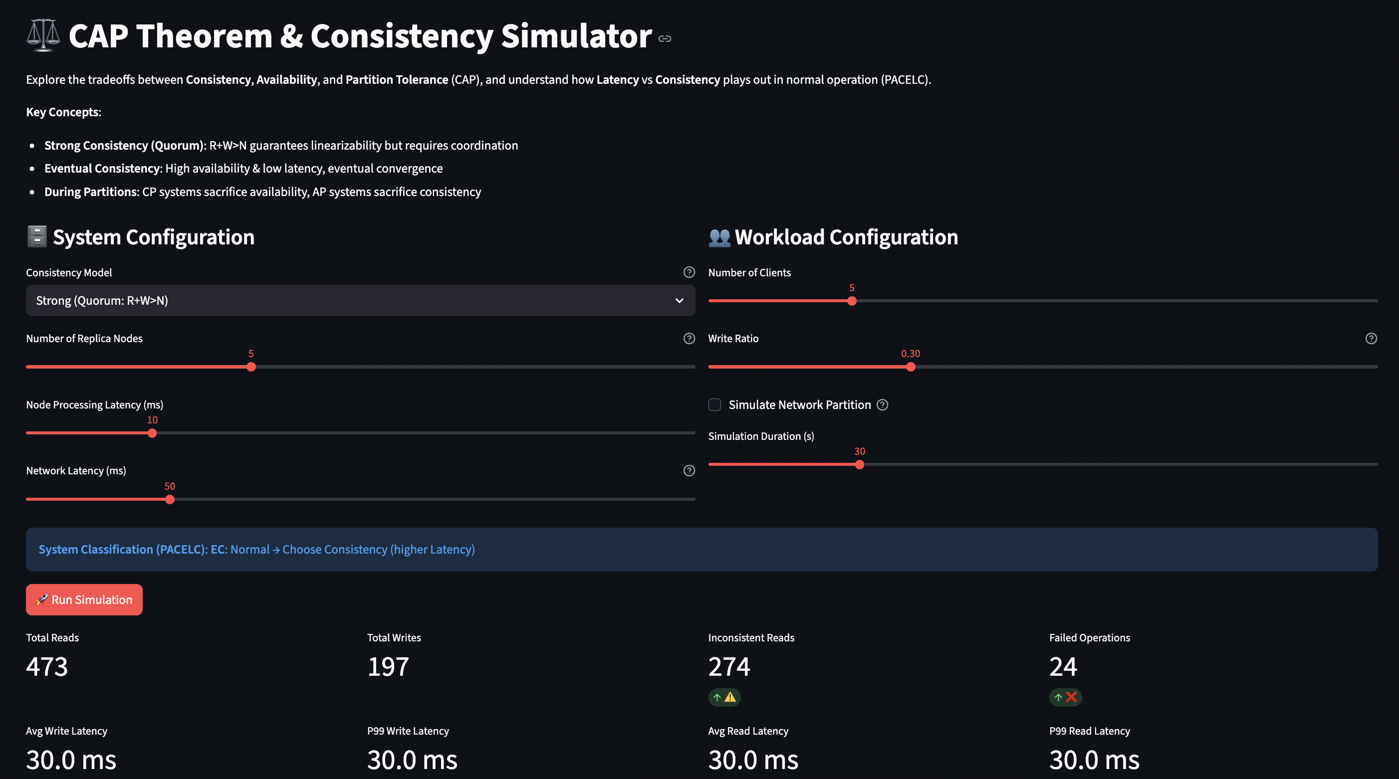
The CAP/PACELC simulator lets you explore these tradeoffs by configuring different consistency models and observing their behavior during normal operation and network partitions.
System Model:
- N replica nodes, each with local storage
- Configurable schema for data (to test compatibility)
- Network latency between nodes (WAN vs LAN)
- Optional partition mode (splits cluster)
Consistency Levels:
- Strong (R+W>N): Quorum reads and writes, linearizable
- Linearizable (R=W=N): All nodes must respond, highest consistency
- Weak (R=1, W=1): Single node, eventual consistency
- Eventual: Async replication, high availability
def get_quorum_size(self, operation_type):
    if self.consistency_level == ConsistencyLevel.STRONG:
        return (self.n_nodes // 2) + 1  # Majority
    elif self.consistency_level == ConsistencyLevel.LINEARIZABLE:
        return self.n_nodes  # All nodes
    elif self.consistency_level == ConsistencyLevel.WEAK:
        return 1  # Any node
Key Parameters:
| Parameter | What It Tests | Impact |
|---|---|---|
n_nodes | Replica count | More nodes = more fault tolerance but higher coordination cost |
consistency_level | Strong/Eventual/etc | Directly controls latency vs consistency tradeoff |
base_latency | Node processing time | Baseline performance |
network_latency | Inter-node delay | WAN (50-150ms) vs LAN (1-10ms) dramatically affects quorum cost |
partition_active | Network partition | Tests CAP behavior (A vs C during partition) |
write_ratio | Read/write mix | Write-heavy shows coordination bottleneck |
What You Can Learn:
- Latency cost of consistency:
- Run with Strong (R=3,W=3) at network_latency=5ms ? ~15ms operations
- Same at network_latency=100ms ? ~300ms operations
- Switch to Weak (R=1,W=1) ? single-digit milliseconds regardless
- CAP during partitions:
- Enable partition with Strong consistency ? operations fail (choosing C over A)
- Enable partition with Eventual ? stale reads but available (choosing A over C)
- Quorum size tradeoffs:
- Linearizable (R=W=N) ? single node failure breaks everything
- Strong (R=W=3 of N=5) ? can tolerate 2 node failures
- Measure failure rate vs consistency guarantees
- Geographic distribution:
- Network latency 10ms (same datacenter) ? quorum cost moderate
- Network latency 150ms (cross-continent) ? quorum cost severe
- Observe when you should use eventual consistency for geo-distribution
The simulator tracks write/read latencies, inconsistent reads, failed operations, and success rates, giving you quantitative data on the tradeoffs.
Key Insights from Simulation
The simulator reveals that most architectural decisions are driven by normal operation latency, not partition handling. If you’re building a global system with 150ms cross-region latency, strong consistency means every operation takes 150ms+ for quorum coordination. That’s often unacceptable for user-facing features. This is why hybrid approaches are becoming standard: use strong consistency for critical invariants (financial transactions, inventory), eventual consistency for everything else (user profiles, preferences).
Part 3: CRDTs
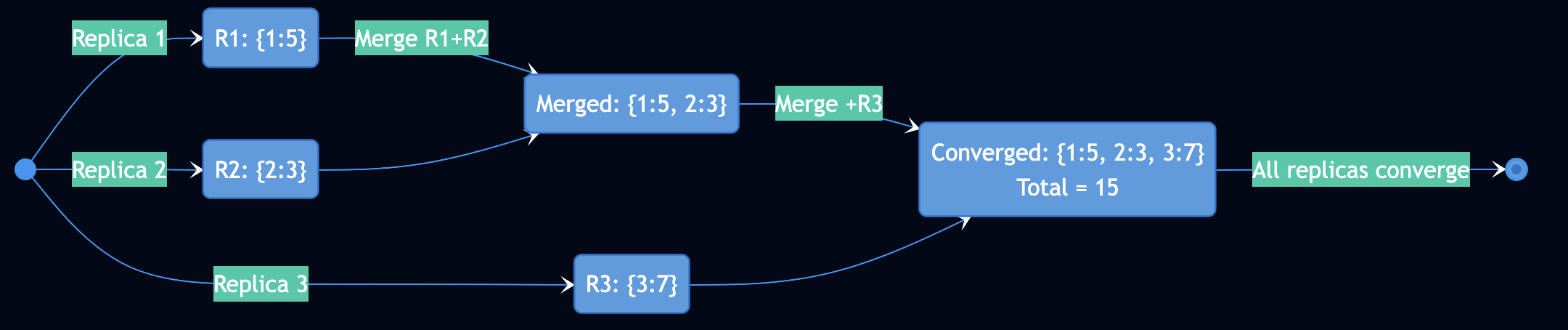
CRDTs (Conflict-Free Replicated Data Types) provide strong eventual consistency (SEC) through mathematical guarantees, not probabilistic convergence. They work without coordination, consensus, or concurrency control. CRDTs rely on operations being commutative (order doesn’t matter), merge functions being associative and idempotent (forming a semilattice), and updates being monotonic according to a partial order.
Example: G-Counter (Grow-Only Counter)
class GCounter:
    def __init__(self, replica_id):
        self.counts = {}  # replica_id -> count

    def increment(self, amount=1):
        # Each replica tracks its own increments
        self.counts[self.replica_id] = self.counts.get(self.replica_id, 0) + amount

    def value(self):
        # Total is sum of all replicas
        return sum(self.counts.values())

    def merge(self, other):
        # Take max of each replica's count
        for replica_id, count in other.counts.items():
            self.counts[replica_id] = max(self.counts.get(replica_id, 0), count)
Why this works:
- Each replica only increments its own counter (no conflicts)
- Merge takes max (idempotent:
max(a,a) = a) - Order doesn’t matter:
max(max(a,b),c) = max(a,max(b,c)) - Eventually all replicas see all increments ? convergence
CRDT Types
There are two main approaches: State-based CRDTs (CvRDTs) send full local state and require merge functions to be commutative, associative, and idempotent. Operation-based CRDTs (CmRDTs) transmit only update operations and require reliable delivery in causal order. Delta-state CRDTs combine the advantages by transmitting compact deltas.
Four CRDTs in the Simulator:
- G-Counter: Increment only, perfect for metrics
- PN-Counter: Increment and decrement (two G-Counters)
- OR-Set: Add/remove elements, concurrent add wins
- LWW-Map: Last-write-wins with timestamps
Production systems using CRDTs include Redis Enterprise (CRDBs), Riak, Azure Cosmos DB for distributed data types, and Automerge/Yjs for collaborative editing like Google Docs. SoundCloud uses CRDTs in their audio distribution platform.
Important Limitations
CRDTs only provide eventual consistency, NOT strong consistency or linearizability. Different replicas can see concurrent operations in different orders temporarily. Not all operations are naturally commutative, and CRDTs cannot solve problems requiring atomic coordination like preventing double-booking without additional mechanisms.
The “Shopping Cart Problem”: You can use an OR-Set for shopping cart items, but if two clients concurrently remove the same item, your naive implementation might remove both. The CRDT guarantees convergence to a consistent state, but that state might not match user expectations.
Byzantine fault tolerance is also a concern as traditional CRDTs assume all devices are trustworthy. Malicious devices can create permanent inconsistencies.
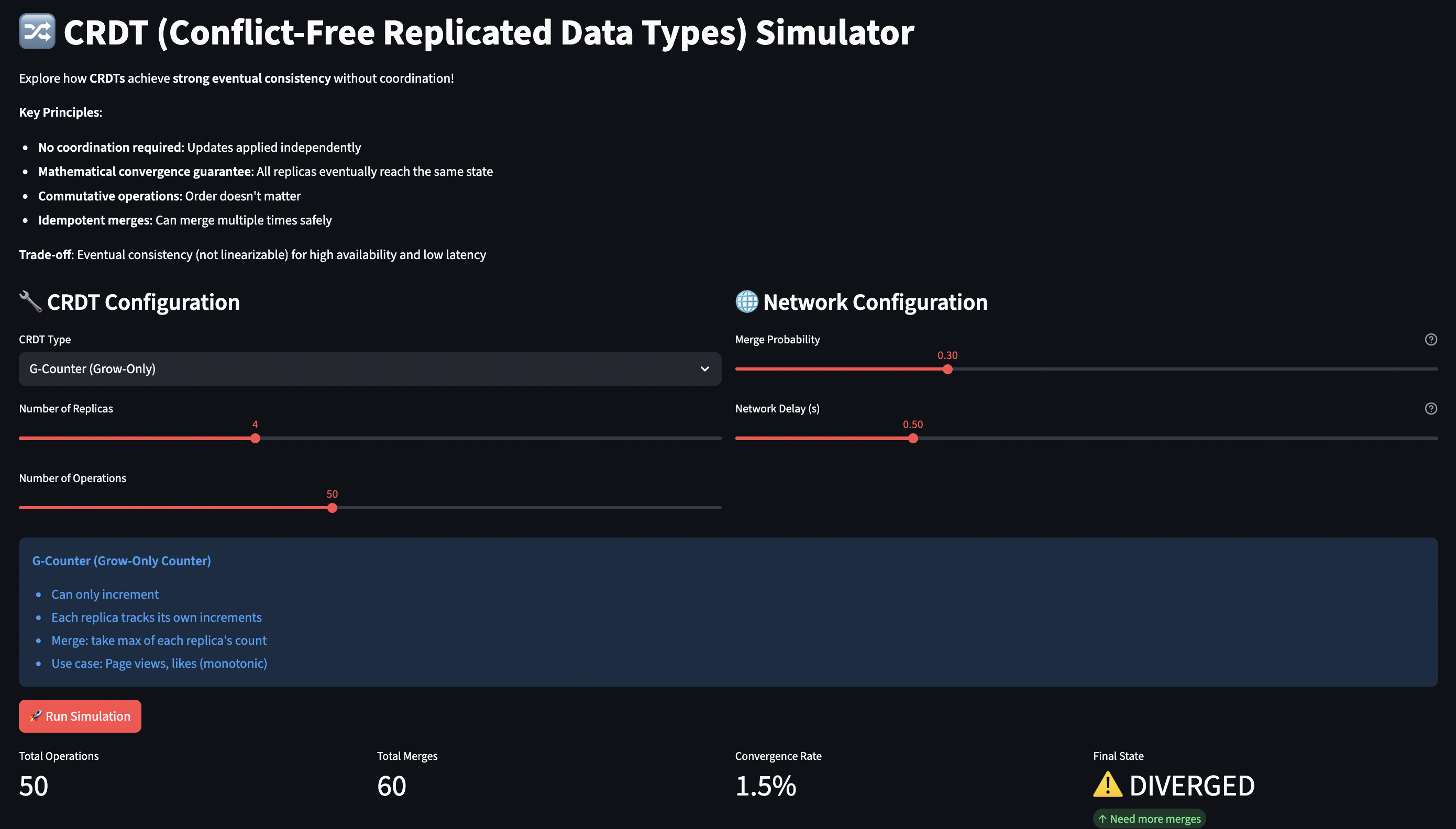
How the Simulator Works
The CRDT simulator demonstrates convergence through gossip-based replication. You can watch replicas diverge and converge as they exchange state.
Simulation Model:
- Multiple replica nodes, each with independent CRDT state
- Operations applied to random replicas (simulating distributed clients)
- Periodic “merges” (gossip protocol) with probability
merge_probability - Network delay between merges
- Tracks convergence: do all replicas have identical state?
CRDT Implementations: Each CRDT type has its own semantics:
# G-Counter: Each replica has its own count, merge takes max
def merge(self, other):
    for replica_id, count in other.counts.items():
        self.counts[replica_id] = max(self.counts.get(replica_id, 0), count)

# OR-Set: Elements have unique tags, add always beats remove
def add(self, element, unique_tag):
    self.elements[element].add(unique_tag)

def remove(self, element, observed_tags):
    self.elements[element] -= observed_tags  # Only remove what was observed

# LWW-Map: Latest timestamp wins
def set(self, key, value, timestamp):
    current = self.entries.get(key)
    if current is None or timestamp > current[1]:
        self.entries[key] = (value, timestamp, self.replica_id)
Key Parameters:
| Parameter | What It Tests | Values |
|---|---|---|
crdt_type | Different convergence semantics | G-Counter, PN-Counter, OR-Set, LWW-Map |
n_replicas | Number of nodes | 2-8 |
n_operations | Total updates | 10-100 |
merge_probability | Gossip frequency | 0.0-1.0 |
network_delay | Time for state exchange | 0.0-2.0s |
What You Can Learn:
- Convergence speed:
- Set merge_probability=0.1 ? slow convergence, replicas stay diverged
- Set merge_probability=0.8 ? fast convergence
- Understand gossip frequency vs consistency window tradeoff
- OR-Set semantics:
- Watch concurrent add/remove ? add wins
- See how unique tags prevent unintended deletions
- Compare with naive set implementation
- LWW-Map data loss:
- Two replicas set same key concurrently with different values
- One value “wins” based on timestamp (or replica ID tie-break)
- Data loss is possible – not suitable for all use cases
- Network partition tolerance:
- Low merge probability simulates partition
- Replicas diverge but operations still succeed (AP in CAP)
- After “partition heals” (merges resume), all converge
- No coordination needed, no operations failed
The simulator visually shows replica states over time and convergence status, making abstract CRDT theory concrete.
Key Insights from Simulation
CRDTs trade immediate consistency for availability and partition tolerance. The theoretical guarantees are proven: if all replicas receive all updates (eventual delivery), they will converge to the same state (strong convergence).
But the simulator reveals the practical challenges:
- Merge semantics don’t always match user intent (LWW can lose data)
- Tombstones can grow indefinitely (OR-Set needs garbage collection)
- Causal ordering adds complexity (need vector clocks for some CRDTs)
- Not suitable for operations requiring coordination (uniqueness constraints, atomic updates)
When to use CRDTs:
- High-write distributed counters (page views, analytics)
- Collaborative editing (where eventual consistency is acceptable)
- Offline-first applications (sync when online)
- Shopping carts (with careful semantic design)
When NOT to use CRDTs:
- Bank account balances (need atomic transactions)
- Inventory (can’t prevent overselling without coordination)
- Unique constraints (usernames, reservation systems)
- Access control (need immediate consistency)
Part 4: Cross-System Interaction (CSI) Failures
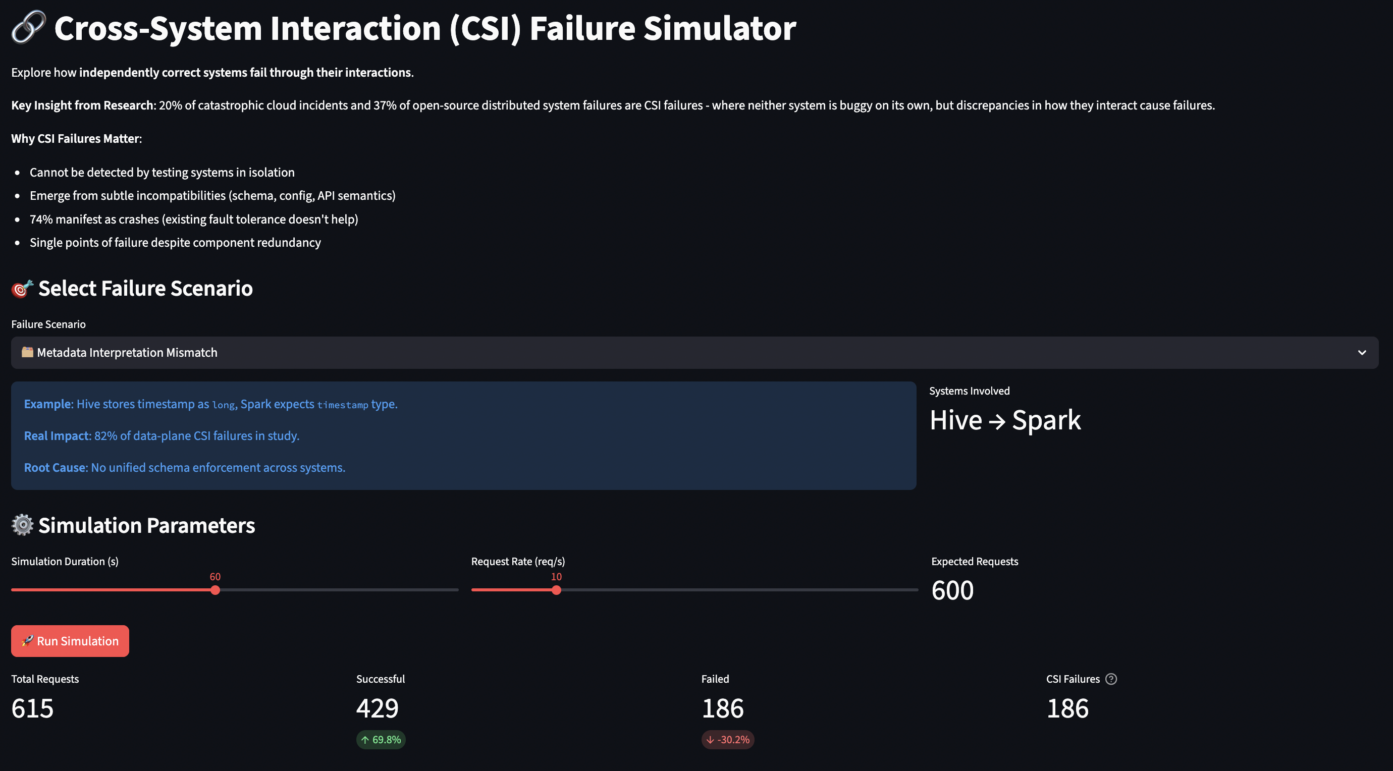
Research from EuroSys 2023 found that 20% of catastrophic cloud incidents and 37% of failures in major open-source distributed systems are CSI failures – where both systems work correctly in isolation but fail when connected. This is the NASA Mars Climate Orbiter problem: one team used metric units, another used imperial. Both systems worked perfectly. The spacecraft burned up in Mars’s atmosphere because of their interaction.
Why CSI Failures Are Different
Not dependency failures: The downstream system is available, it just can’t process what upstream sends.
Not library bugs: Libraries are single-address-space and well-tested. CSI failures cross system boundaries where testing is expensive.
Not component failures: Each system passes its own test suite. The bug only emerges through interaction.
CSI failures manifest across three planes: Data plane (51% – schema/metadata mismatches), Management plane (32% – configuration incoherence), and Control plane (17% – API semantic violations).
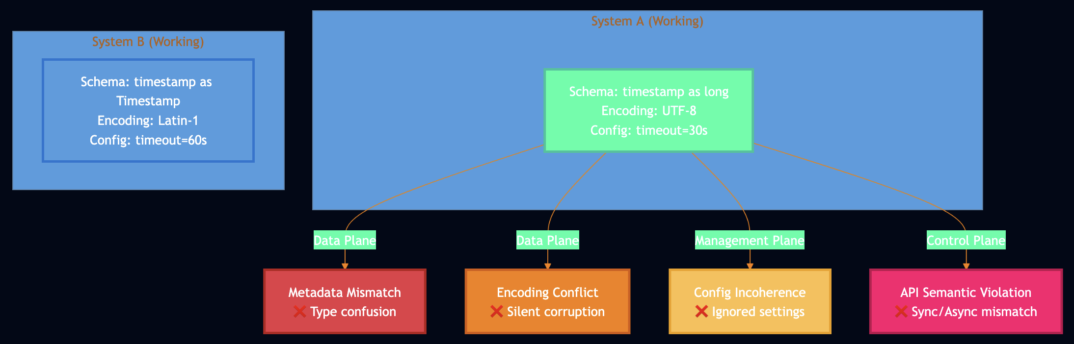
For example, study of Apache Spark-Hive integration found 15 distinct discrepancies in simple write-read testing. Hive stored timestamps as long (milliseconds since epoch), Spark expected Timestamp type. Both worked in isolation, failed when integrated. Kafka and Flink encoding mismatch: Kafka set compression.type=lz4, Flink couldn’t decompress due to old LZ4 library. Configuration was silently ignored in Flink, leading to data corruption for 2 weeks before detection.
Why Testing Doesn’t Catch CSI Failures
Analysis of Spark found only 6% of integration tests actually test cross-system interaction. Most “integration tests” test multiple components of the same system. Cross-system testing is expensive and often skipped. The problem compounds with modern architectures:
- Microservices: More system boundaries to test
- Multi-cloud: Different clouds with different semantics
- Serverless: Fine-grained composition increases interaction surface area
How the Simulator Works
The CSI failure simulator models two systems exchanging data, with configurable discrepancies in schemas, encodings, and configurations.
System Model:
- Two systems (upstream ? downstream)
- Each has its own schema definition (field types, encoding, nullable fields)
- Each has its own configuration (timeouts, retry counts, etc.)
- Data flows from System A to System B with potential conversion failures
Failure Scenarios:
- Metadata Mismatch (Hive/Spark):
- System A:
timestamp: long - System B:
timestamp: Timestamp - Failure: Type coercion fails ~30% of the time
- System A:
- Schema Conflict (Producer/Consumer):
- System A:
encoding: latin-1 - System B:
encoding: utf-8 - Failure: Silent data corruption
- System A:
- Configuration Incoherence (ServiceA/ServiceB):
- System A:
max_retries=3, timeout=30s - System B expects:
max_retries=5, timeout=60s - Failure: ~40% of requests fail due to premature timeout
- System A:
- API Semantic Violation (Upstream/Downstream):
- Upstream assumes: synchronous, thread-safe
- Downstream is: asynchronous, not thread-safe
- Failure: Race conditions, out-of-order processing
- Type Confusion (SystemA/SystemB):
- System A:
amount: float - System B:
amount: decimal - Failure: Precision loss in financial calculations
- System A:
Implementation Details:
class DataSchema:
    def __init__(self, schema_id, fields, encoding, nullable_fields):
        self.fields = fields  # field_name -> type
        self.encoding = encoding

    def is_compatible(self, other):
        # Check field types and encoding
        return (self.fields == other.fields and
                self.encoding == other.encoding)

class DataRecord:
    def serialize(self, target_schema):
        # Attempt type coercion
        for field, value in self.data.items():
            expected_type = target_schema.fields[field]
            actual_type = self.schema.fields[field]

            if expected_type != actual_type:
                # 30% failure on type mismatch (simulating real world)
                if random.random() < 0.3:
                    return None  # Serialization failure

        # Check encoding compatibility
        if self.schema.encoding != target_schema.encoding:
            if random.random() < 0.2:  # 20% silent corruption
                return None
Key Parameters:
| Parameter | What It Tests |
|---|---|
failure_scenario | Type of CSI failure (metadata, schema, config, API, type) |
duration | Simulation length |
request_rate | Load (requests per second) |
The simulator doesn’t have many tunable parameters because CSI failures are about specific incompatibilities, not gradual degradation. Each scenario models a real-world pattern.
What You Can Learn:
- Failure rates: CSI failures often manifest in 20-40% of requests (not 100%)
- Some requests happen to have compatible data
- Makes debugging harder (intermittent failures)
- Failure location:
- Research shows 69% of CSI fixes go in the upstream system, often in connector modules that are less than 5% of the codebase
- Simulator shows which system fails (usually downstream)
- Silent vs loud failures:
- Type mismatches often crash (loud, easy to detect)
- Encoding mismatches corrupt silently (hard to detect)
- Config mismatches cause intermittent timeouts
- Prevention effectiveness:
- Schema registry eliminates metadata mismatches
- Configuration validation catches config incoherence
- Contract testing prevents API semantic violations
Key Insights from Simulation
The simulator demonstrates that cross-system integration testing is essential but often skipped. Unit tests of each system won’t catch these failures.
Prevention strategies validated by simulation:
- Write-Read Testing: Write with System A, read with System B, verify integrity
- Schema Registry: Single source of truth for data schemas, enforced across systems
- Configuration Coherence Checking: Validate that shared configs match
- Contract Testing: Explicit, machine-checkable API contracts
Hybrid Consistency Models
Modern systems increasingly use mixed consistency: RedBlue Consistency (2012) marks operations as needing strong consistency (red) or eventual consistency (blue). Replicache (2024) has the server assign final total order while clients do optimistic local updates with rebase. For example: Calendar Application
# Strong consistency for room reservations (prevent double-booking)
def book_conference_room(room_id, time_slot):
    with transaction(consistency='STRONG'):
        if room.is_available(time_slot):
            room.book(time_slot)
            return True
        return False

# CRDTs for collaborative editing (participant lists, notes)
def update_meeting_notes(meeting_id, notes):
    # LWW-Map CRDT, eventual consistency
    meeting.notes.merge(notes)

# Eventual consistency for preferences
def update_user_calendar_color(user_id, color):
    # Who cares if this propagates slowly?
    user_prefs[user_id] = color
Recent theoretical work on the CALM theorem proves that coordination-free consistency is achievable for certain problem classes. Research in 2025 provided mathematical definitions of when coordination is and isn’t required, separating coordination from computation.
What the Simulators Teach Us
Running all four simulators reveals the consistency spectrum:
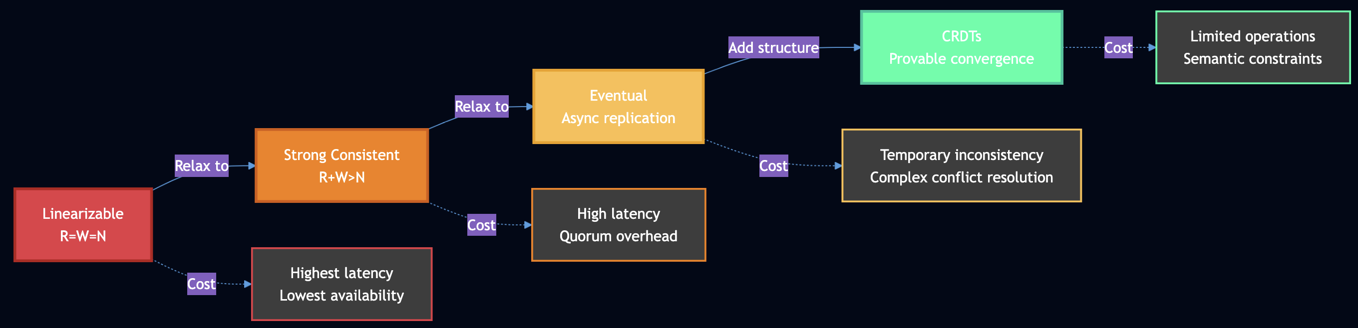
No “best” consistency model exists:
- Quorums are best when you need linearizability and can tolerate latency
- CRDTs are best when you need high availability and can tolerate eventual consistency
- Neither approach “bypasses” CAP – they make different tradeoffs
- Real systems use hybrid models with different consistency for different operations
Practical Lessons
1. Design for Recovery, Not Just Prevention
The metastable failure simulator shows you can’t prevent all failures. Your retry logic, backoff strategy, and circuit breakers are more important than your happy path code. Validated strategies include:
- Exponential backoff with jitter (spread retries over time)
- Adaptive retry budgets (limit total fleet-wide retries)
- Circuit breakers (detect patterns, stop storms)
- Load shedding (fail fast rather than queue to death)
2. Understand the Consistency Spectrum
The CAP/PACELC simulator demonstrates that consistency is not binary. You need to understand:
- What consistency level do you actually need? (Most operations don’t need linearizability)
- What’s the latency cost? (Quorum reads in cross-region deployment can be 100x slower)
- What happens during partitions? (Can you sacrifice availability or must you serve stale data?)
Decision framework:
- Use strong consistency for: money, inventory, locks, compliance
- Use eventual consistency for: feeds, catalogs, analytics, caches
- Use hybrid models for: most real-world applications
3. Test Cross-System Interactions
The CSI failure simulator reveals that 86% of fixes go into connector modules that are less than 5% of your codebase. This is where bugs hide. Essential tests include:
- Write-read tests (write with System A, read with System B)
- Round-trip tests (serialize/deserialize across boundaries)
- Version compatibility matrix (test combinations)
- Schema validation (machine-checkable contracts)
4. Leverage CRDTs Where Appropriate
The CRDT simulator shows that conflict-free convergence is possible for specific problem types. But you need to:
- Understand the semantic limitations (LWW can lose data)
- Design merge behavior carefully (does it match user intent?)
- Handle garbage collection (tombstones, vector clocks)
- Accept eventual consistency (not suitable for all use cases)
5. Monitor for Sustaining Effects
Metastability, retry storms, and goodput collapse are self-sustaining failure modes. They persist after the trigger is gone. Critical metrics include:
- P99 latency vs timeout threshold (approaching timeout = danger)
- Retry rate vs success rate (high retries = storm risk)
- Queue depth (unbounded growth = admission control needed)
- Goodput vs throughput (doing useful work vs spinning)
Using the Simulators
All four simulators are available at: https://github.com/bhatti/simulators
Installation
git clone https://github.com/bhatti/simulators
cd simulators
pip install -r requirements.txt
Requirements:
- Python 3.7+
- streamlit (web UI)
- simpy (discrete event simulation)
- plotly (interactive visualizations)
- numpy, pandas (data analysis)
Running Individual Simulators
# Metastable failure simulator
streamlit run metastable_simulator.py

# CAP/PACELC consistency simulator
streamlit run cap_consistency_simulator.py

# CRDT simulator
streamlit run crdt_simulator.py

# CSI failure simulator
streamlit run csi_failure_simulator.py
Running All Simulators
python run_all_simulators.py
Conclusion
Building distributed systems means confronting failure modes that are expensive or impossible to reproduce in real environments:
- Metastable failures require specific load patterns and timing
- Consistency tradeoffs need multi-region deployments to observe
- CRDT convergence requires orchestrating concurrent operations across replicas
- CSI failures need exact schema/config mismatches that don’t exist in test environments
Simulators bridge the gap between theoretical understanding and practical intuition:
- Cheaper than production testing: No cloud costs, no multi-region setup, instant feedback
- Safer than production experiments: Crash the simulator, not your service
- More complete than unit tests: See emergent behaviors, not just component correctness
- Faster iteration: Tweak parameters, re-run in seconds, build intuition through experimentation
What You Can’t Learn Without Simulation
- When does retry amplification tip into metastability? (Depends on coordination slope, timeout, backoff)
- How much does quorum coordination actually cost? (Depends on network latency, replica count, workload)
- Do your CRDT semantics match user expectations? (Depends on merge behavior, conflict resolution)
- Will your schema changes break integration? (Depends on type coercion, encoding, version skew)
The goal isn’t to prevent all failures, that’s impossible. The goal is to understand, anticipate, and recover from the failures that will inevitably occur.
References
Key research papers and resources used in this post:
- AWS Metastability Research (HotOS 2025) – Sustaining effects and goodput collapse
- Marc Brooker on DSQL – Practical distributed SQL considerations
- James Hamilton on Reliable Systems – Large-scale system design
- CSI Failures Study (EuroSys 2023) – Cross-system interaction failures
- PACELC Framework – Beyond CAP theorem
- Marc Brooker on CAP – CAP theorem revisited
- Anna CRDT Database – Autoscaling with CRDTs
- Linearizability Paper – Herlihy & Wing’s foundational work
- Designing Data-Intensive Applications by Martin Kleppmann
- Distributed Systems Reading Group – MIT CSAIL
- Jepsen.io – Kyle Kingsbury’s consistency testing
- Aphyr’s blog – Distributed systems deep dives